Portfolio Optimization- Modern Portfolio Theory
Introduction
Our University Endowment Fund employs portfolio theory to determine the optimal portfolio. We have constructed a well-diversified portfolio consisting of 13 different asset classes to maximize the reward-to-risk ratio. These asset classes include US large-cap stocks, US small-cap stocks, developed market equities, emerging market equities, commodities, US real estate, T-bills, US treasury bonds, US investment-grade corporate bonds, US high-yield bonds, global high-yield bonds, global high-yield corporate bonds, and global treasury bonds.
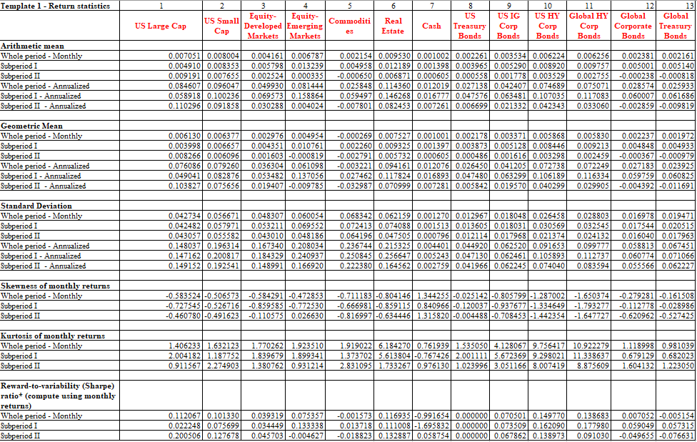
The portfolio analysis process begins by assessing the risk and return relationship. To estimate future rates of return and determine appropriate levels of risk, we have utilized 20 years of historical data for all 13 asset classes. While our analysis assumes a normal distribution of data, we have also considered any deviations from normality by examining the skewness and kurtosis of the data to account for potential asymmetry and the probability of extreme returns.
Modern Portfolio Theory, based on the principle of diversification, guides our approach. Developed by Harry Markowitz, the theory emphasizes the importance of not putting all our eggs in one basket. We seek to efficiently diversify our portfolio by identifying the efficient set of portfolios. By employing Markowitz’s theory, we can determine the highest level of return for a given level of risk. We have conducted various analyses using 23 different models, incorporating factors such as changes in interest rates, investment constraints, and different target returns. Additionally, we have explored the applicability of optimal weights from previous periods to assess their relevance for the future. By employing this comprehensive approach, our University Endowment Fund strives to construct an optimal portfolio that balances risk and reward while maximizing returns for our stakeholders.
Naïve Diversification VS Efficient diversification
An equal-weighted portfolio increases the risks of securities stocks in the investment portfolio of an investor. Risk in such a portfolio cannot be eliminated easily because diversification is not possible. The value of an investment portfolio may decline over a given time period simply because of economic changes or other events (change in tax reforms, change in the world energy situation, etc.) that impact large portions of the market.
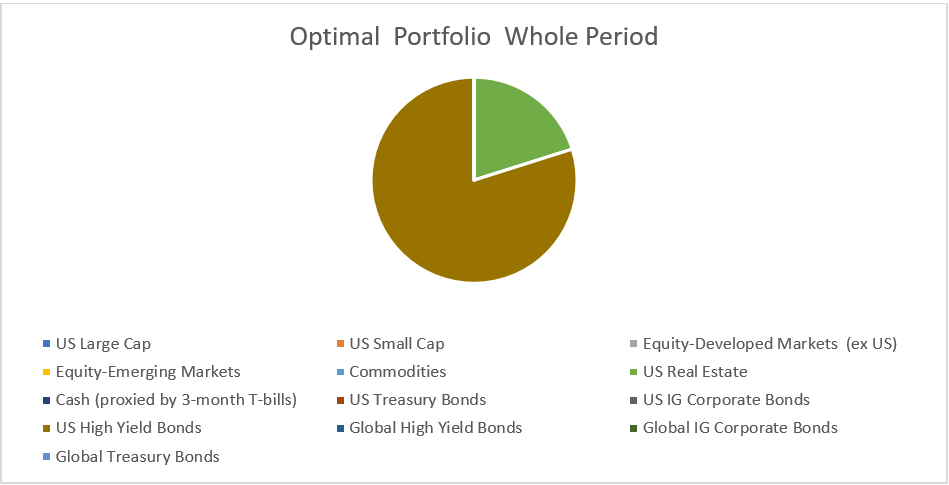
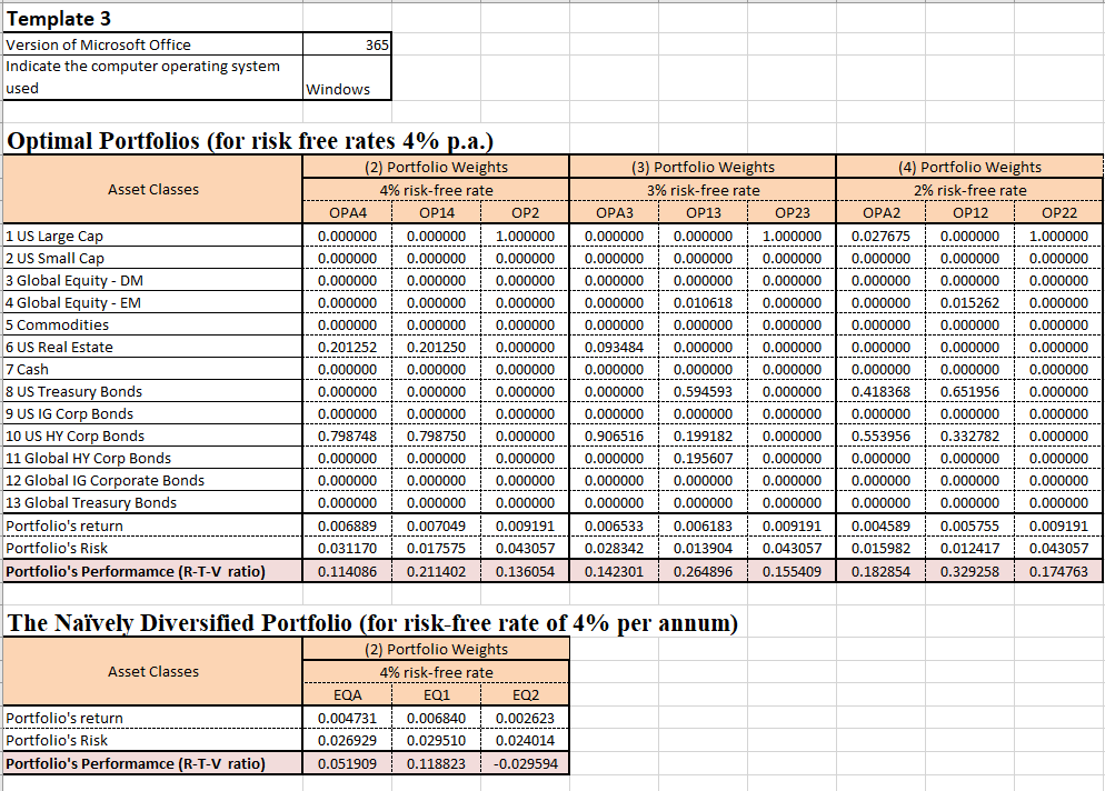
Figure 1: Optimal Portfolio Whole Period
The Optimal Portfolio (OPA), which is constructed based on the mean-variance optimization technique, aims to achieve the highest possible return for a given level of risk. In our case, the OPA had a risk of 3.117% and a return of 0.689%. This means that the OPA was able to generate a relatively higher return for the level of risk taken. As we can see from Figure 1 the OPA is able to generate a higher return by investing 20% of our assets in Real estate and 80% of our assets in US high-yield bonds.
On the other hand, the EQA, which involves allocating equal weights to all assets in the portfolio, had a lower risk of 2.693% but also a lower return of 0.473%. The equal-weighted approach assumes that all assets in the portfolio have an equal contribution to the overall performance. The difference in performance between the EQA and OPA can be attributed to several factors. One factor is that the assets in the portfolio had varying levels of risk and return, which were not considered in the equal-weighted approach. By assigning equal weights to all assets, the EQA has been overexposed to lower-performing assets and underexposed to higher-performing assets, resulting in a lower overall return.
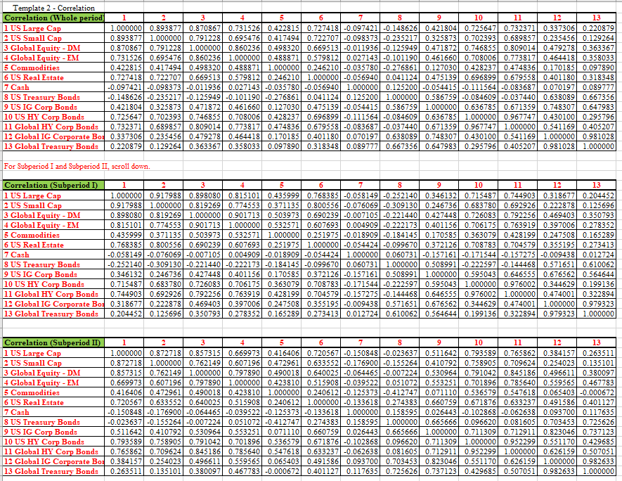
Furthermore, the OPA takes into account the correlation between assets, allowing for diversification benefits. This means that the OPA is able to construct a portfolio that minimizes risk by selecting assets that have a lower correlation with each other. The EQA, on the other hand, does not consider correlations and may not have achieved the same level of diversification.
Difference between Sub-Periods
During sub-period 1, the portfolio had a greater emphasis on US Real Estate (20.1252%) and US High-Yield Corporate Bonds (79.8748%). This allocation indicates that the real estate market may have experienced advantageous conditions, including factors like low-interest rates, heightened demand or optimistic performance expectations. Investors likely expected superior returns from US Real Estate in comparison to alternative asset classes. One of the interesting economic events during this period was the 2008 financial crisis which had a significant effect on the US market.
In sub-period 2, the portfolio weights demonstrate a complete shift from US Real Estate and US High-Yield Corporate Bonds. The entire allocation is focused solely on US Large Cap Equities (100%). This indicates that during sub-period 2, the prevailing economic environment and market conditions were favorable for Large-Cap US Equities, making them the most attractive investment choice. Several factors could have contributed to the shift toward US Large Cap Equities in subperiod 2. During that time, the stock market experienced a bullish trend, demonstrating robust performance. The allocation might also reflect the expectation of greater returns from US Large Cap Equities compared to other asset classes, driven by factors like encouraging economic indicators.
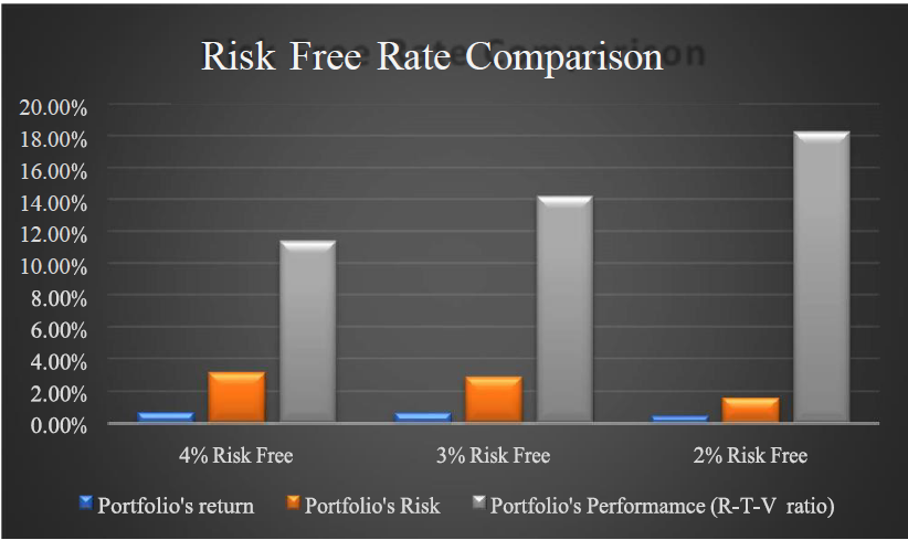
Difference Between Risk-Free Rates
A downward change in the risk-free rate would have a positive effect on portfolio performance. As the risk-free rate decreases it becomes easier for companies to be able to borrow money at a better rate. This is shown in our portfolio performance when we adjust the risk-free rate. If we look at our OPA4 portfolio we can see that with a 4% risk-free rate we have a monthly return of .6889% and an RTV ratio of .114, when we reduce the risk-free rate to 3% in OPA3 we get a return of .6533% and an RTV ratio of .142, when we reduce the risk-free rate further to 2% in OPA2 we get a return of .4589% and a RTV ratio of .183. These scenarios all show a slight decrease in the expected return because of the decline in the risk-free rate but the risk-adjusted performance is actually better because when the portfolio return has the risk-free rate subtracted the risk-free rate is smaller.
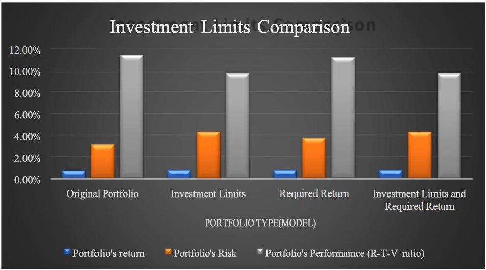
Adding Investment Limits and Target Return
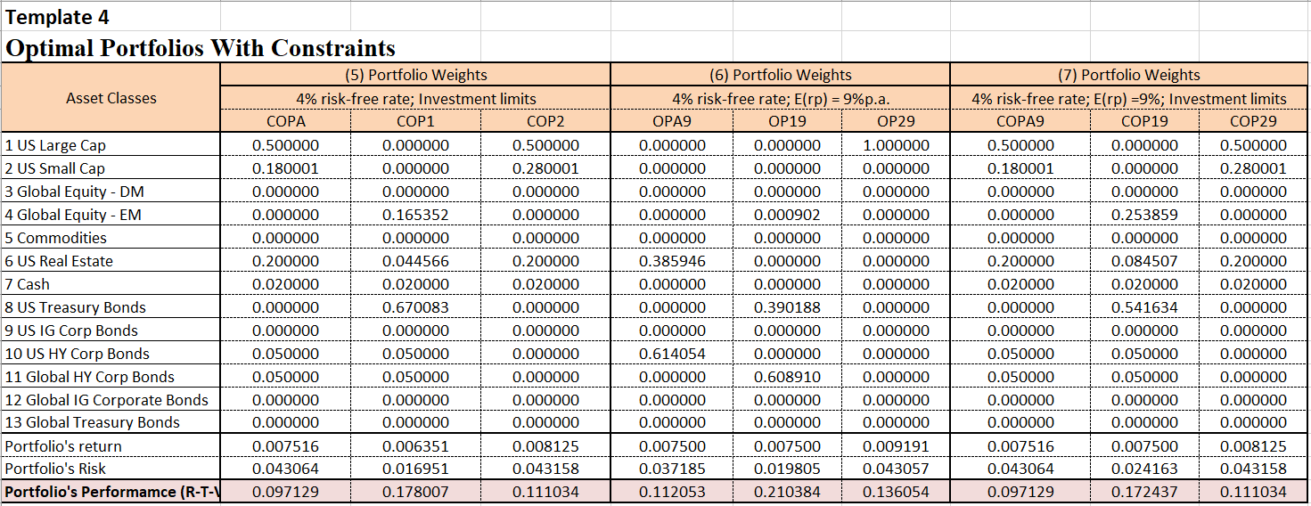
Adding investment limits to our portfolio or adding a 9% return target will cause some detrimental effects on our portfolio. Starting with the investment limits when we compare our limited portfolio in COPA to our original OPA4 portfolio we see a 9.1% increase in required return but a 14.9% decrease in RTV. This is due to the increase in risk from adding the investment limits. When we look at the combined investment limit and target required return portfolio COPA9 there is a 9.1% decrease in return and a 14.9% decrease in RTV. These results indicate that although we may see some increased return when adding these investment limits this is at the cost of significantly increased risk and decrease in RTV ratio. Based on these results I would not recommend adding these investment limitations without specific reasons for a required return amount or asset allocation limitations.

Sensitivity to Changing Interest Rates
The mean-optimization is indeed sensitive to changing the targeted level of risk because our analysis is based on Markowitz portfolio theory which is to determine the highest level of return for a given level of risk. What we have done in our analysis is an alternative approach that is we have found the portfolio with the least amount of risk for the given level of return, no matter what route we take the result would be the same as both those routes would derive the same efficient frontier. To prove this point we have run our model without any constraint or targeted return and with a constraint or a targeted return of 9% (0.75% monthly). Table 1 demonstrates the sensitivity of portfolio risk by comparing the risk and return of both models – the one with the target return constraint and the one without it. The table highlights that each model produces different levels of risk and, in some cases, different returns. Even when the return is the same, we observe that the portfolio’s risk is influenced by the presence of a constraint. For instance, consider the cases of COPA9 and COPA for the entire period. The model without the constraint already yielded a return higher than the target return, making it the optimal risky portfolio for the given target. Therefore, the combination of assets remains unchanged in this scenario.
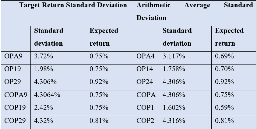
Table 1 compares Target and Arithmetic average return models
Overall, our analysis confirms that the mean-optimization approach is sensitive to the chosen level of risk constraint. By examining the risk and return trade-offs in different portfolios, we gain valuable insights into portfolio construction and the impact of targeting specific returns on risk levels.
Out-of-Sample Test Results
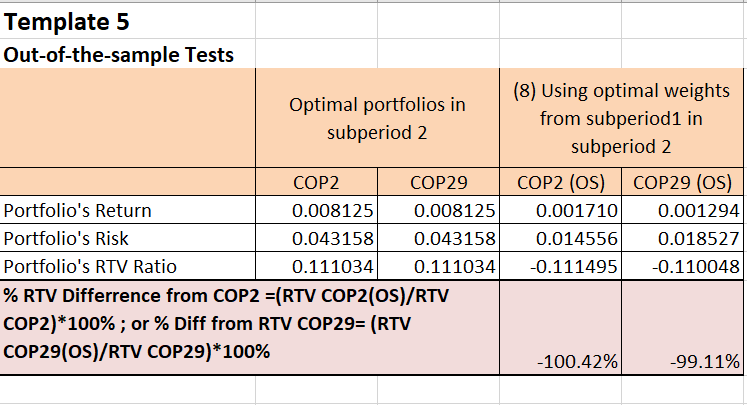
Although using the optimal weights from previous periods can be used as a reference or setting expectations for the future performance of a portfolio it doesn’t necessarily mean that it will be the optimal weight of a portfolio in the future. There are a few reasons as to why this may not be the case. First, the market conditions of the past will not be the same as the market conditions in the future therefore we can not replicate the same exact returns. Portfolio optimization relies on the expected return, risk, correlation among different assets, and the risk-free rate, all those factors are difficult to predict and are subject to change any time therefore a single change in those factors can also change the outcome of the optimal portfolio. Second, the investors’ objectives might also change during a given period therefore the new portfolio might have new constraints that will change the optimal weight of the portfolio. In our analysis, we have done out of sample results to see if the optimal weight from sub-period one would give us a better return to volatility ratio in the second period, and those results are described in
.png)
Table 2. Table 2 Out of sample and Optimal Portfolio Model
As we can see from the table both the portfolios using the mean-variance allocation have a higher Sharpe ratio and a higher reward. COP2 which is the portfolio for subperiod 2 uses the optimal weight from subperiod one and it has a return of 0.17%, standard deviation of 1.45%, and Reward volatility ratio of -0.1115 while COP2 the optimal portfolio using the mean-variance optimization model gives us a return of 0.81%, standard deviation of 4.33% and positive reward to volatility ratio of 0.11. this is also true for subperiod 2 with constraints, the optimal portfolio gives us a reward-to-volatility ratio of 0.11 while using the optimal period from subperiod one gives us a negative reward-to-volatility ratio of -0.11. investors prefer a portfolio with the highest possible reward for a given level of volatility as we can see from COP2(OS) the reward to volatility is negative therefore it is not the optimal weight.
Conclusion
Our analysis has helped us determine an optimal portfolio for our asset classes, while also allowing us to see what would happen if we adjusted our inputs and requirements. Some of our key findings were that naive diversification yields less positive returns than the optimally diversified portfolio which is reasonable given the naïve portfolio will have allocations in asset classes which may not give us the best results in our overall portfolio. We also can see that the different subperiods have very different results, this is due to different economic circumstances in the 2003-2012 range of subperiod 1 and the 2013-2022 range of subperiod 2, subperiod 1 included the economic crisis of 2008 and subperiod 2 included the COVID crisis. Both economic events had different effects on the economy, so it stands to reason that the subperiods would yield significantly different results. When we analyze the effect of the risk-free rate we see that a decrease in the risk-free rate will have a positive effect on the RTV performance of our portfolios, so we should see an increase in performance if the rates drop/the rate hikes stop. We have also assessed our performance when investment allocation limits and a target return rate are provided, we determined that these will have a negative effect on our performance as these extra conditions don’t allow us to optimize our portfolio as efficiently as possible. Finally, we also saw the results of using portfolio weights from different subperiods in other subperiods (out-of-sample results) this clearly causes detrimental results as the optimization allocations are very dependent on the performance of the asset classes in specific periods so when using a different period’s optimal allocations weights, we won’t yield similar results. Overall, we learned the effects of different alterations to our optimal portfolio model and figured out how to build a portfolio using numerous asset classes as efficiently as possible.
Appendix